


LINKED PAPER
Comparing migratory connectivity across species: The importance of considering the pattern of sampling and the processes that lead to connectivity. Cresswell, W., Patchett, R. 2023. IBIS. DOI: 10.1111/ibi.13261. VIEW
Migratory connectivity seems like quite a good and simple idea. A population of migrants breeds here and winters there. Join the dots and you have connectivity. You know where a breeding population goes, giving you a greater understanding of the species’ behavioural ecology, and you can focus your conservation efforts in the right places. But can we measure the degree to which one breeding population might go to a specific and unique non-breeding area (high connectivity), or where different populations might end up in the same non-breeding area (low connectivity), and so compare connectivity across populations and species? What if describing a species as having high or low connectivity was determined by context: by whether you were interested in describing distributions or the theoretical basis of connectivity? And what if most conclusions of high or low connectivity were dependant on the pattern of sampling rather than the actual traits of individual species?
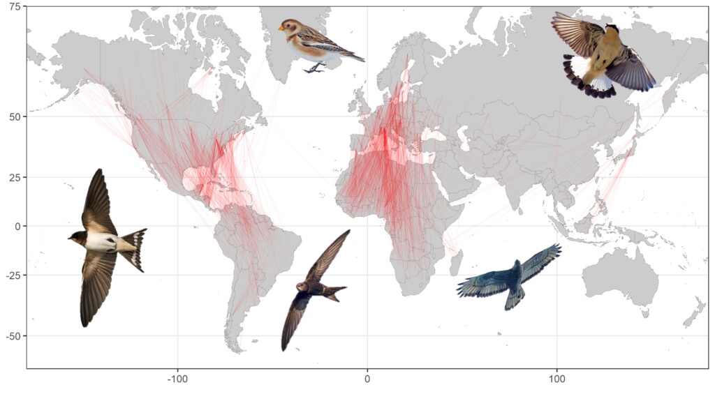
Figure 1. The start and end of 1813 migratory tracks from the 101 landbird species from 127 tracking studies used to work out whether measures of migratory connectivity are comparative. All landbird tracking studies that could be found in the literature up to July 2019 are included in this map. Inset images © John Anderson.
The main issue is sometimes we are just trying to describe connectivity, whereas other times we are trying to understand how connectivity arises and its flexibility in the face of global change. This is best illustrated with an example. Consider the distribution of the Lesser Kestrel in Europe and Africa. All European breeding populations have now been tracked and their non-breeding areas mapped. There is observed high connectivity because Iberian populations spend the non-breeding season in West Africa and Greek populations in Central Africa. But from an evolutionary perspective, Lesser Kestrels tend towards low potential connectivity. They have a fairly average migratory spread – the degree to which any population of Lesser Kestrels spreads out on the non-breeding grounds is only a few percent lower than the average spread measured in 86 species (sampled from many families and three different flyways). The current, observed non-breeding distribution is therefore largely a consequence of the breeding distribution, and Lesser Kestrels simply migrate approximately south. Clearly from a current conservation point of view, Iberian populations are best served by policies targeted towards West Africa, and Greek populations by policies targeted towards Central Africa. Yet from a long-term evolutionary point of view, Lesser Kestrels are a typical generalist, bet-hedging migrant spreading out widely from its breeding site finding any suitable habitat available to the south in Africa. So as the distribution of this habitat shifts – and this happens every decade or so in Africa – some of the population will find and use this habitat leading to a shift in its non-breeding distribution. At the present time, there is habitat more or less directly to the south of all populations, so there has been no selection for targeted dispersal, and flexibility likely remains in the population to adapt to shifting locations of habitat. So the context of what we are using connectivity for determines its level – high connectivity for Lesser Kestrels from a Spanish or Greek conservation point of view – but low connectivity from an evolutionary or climatic flexibility point of view.

Figure 2. Male Lesser Kestrel, a migrant with high connectivity from a conservation perspective, but low connectivity from an evolutionary perspective © John Anderson.
There is another big confusion when defining connectivity or comparing connectivity across species that arises from a disregard of the spatial pattern of sampling of breeding populations. Consider another example. If we track Barn Swallows from a population in North America and one in Europe we can conclude (unsurprisingly) there is high connectivity because there is no overlap in wintering populations in the two different continental flyways. But if we track a population from Berlin and one from London, we would conclude there is low connectivity because swallows from both populations end up overlapping right across Africa, from Accra to Cape Town. If you measure the migratory spread of all these global populations you would find they all have similar values. That swallows that start migrating very far apart, are never likely to overlap on their non-breeding ground seems obvious put this way. Yet the literature is full of statements of species having low or high connectivity without controlling for the spatial pattern of sampling. Even sophisticated measures of connectivity, such as the widely used Mantel correlation coefficient, which apparently gives a solid, objective number on a scale of 0 to 1, suffers from this problem.

Figure 3. Barn Swallow, a migrant with any level of connectivity you like depending on the degree of spatial separation of the breeding populations tracked, and the sample size of the study. But, a consistent very low connectivity in terms of its migratory spread, regardless of how populations are sampled © John Anderson.
A final big problem in measuring connectivity is sample size. Studies with small sample size inevitably show higher connectivity because they sample only a relatively small range for a species. And most connectivity data comes from tracking studies where sample sizes are notoriously small because of the expense and difficulties in tracking large and small birds respectively.
The solution is to be clear about the terms and conditions of any migratory connectivity study, and in particular to be careful about whether we are simply describing the current snapshot of migratory populations’ distribution or whether we are measuring the connectivity processes that gives rise to these snapshots. Migratory spread – the average spacing in the non-breeding area between any pair of individuals from the same tracked breeding population – is one way to keep things simple. All things being equal, a species such as an Ortolan Bunting that has low migratory spread will inevitably have higher connectivity: a species such as a Barn Swallow that has high migratory spread will inevitably have lower connectivity. And because migratory spread cannot be confounded by the spatial distribution of sampled populations, it is measured at the level of the individual, and relatively robust to sample size, it can be compared meaningfully between studies, populations and species.
When we use a truly comparative measure of connectivity, we can look for general patterns across species. Then we find that most migrants are similar in their large migratory spread. Only a few species have specialised to have localised, specific non-breeding sites. Most have remained flexible, spreading out widely, the better to bet hedge against often unpredictable conditions on the non-breeding ground. Which means that most migrant species are already pre-adapted to track the changing distribution of climate and habitat in the Anthropocene. The next question is then – can they track the changes fast enough?
Image credits
Top right: European Bee-eater, a species with a reasonably average high migratory spread so well adapted to find and use new areas of Africa (and indeed Europe as this year’s breeders in the UK demonstrate) as they become suitable because of climate change. High levels of migratory spread in most migrant species suggests that habitat shift due to climate change is not the main driver of their declines © John Anderson.
Blog posts express the views of the individual author(s) and not those of the BOU.
If you want to write about your research in #theBOUblog, then please see here